Version information

%matplotlib inline
from PySide2.QtWidgets import *
from datetime import date
print("Running date:", date.today().strftime("%B %d, %Y"))
import pyleecan
print("Pyleecan version:" + pyleecan.__version__)
import SciDataTool
print("SciDataTool version:" + SciDataTool.__version__)

Running date: April 27, 2023
Pyleecan version:1.5.0
SciDataTool version:2.5.0

How to define a simulation to call FEMM

This tutorial shows the different steps to compute magnetic flux and electromagnetic torque with Pyleecan automated coupling with FEMM. This tutorial was tested with the release 21Apr2019 of FEMM. Please note that the coupling with FEMM is only available on Windows.

The notebook related to this tutorial is available on GitHub.

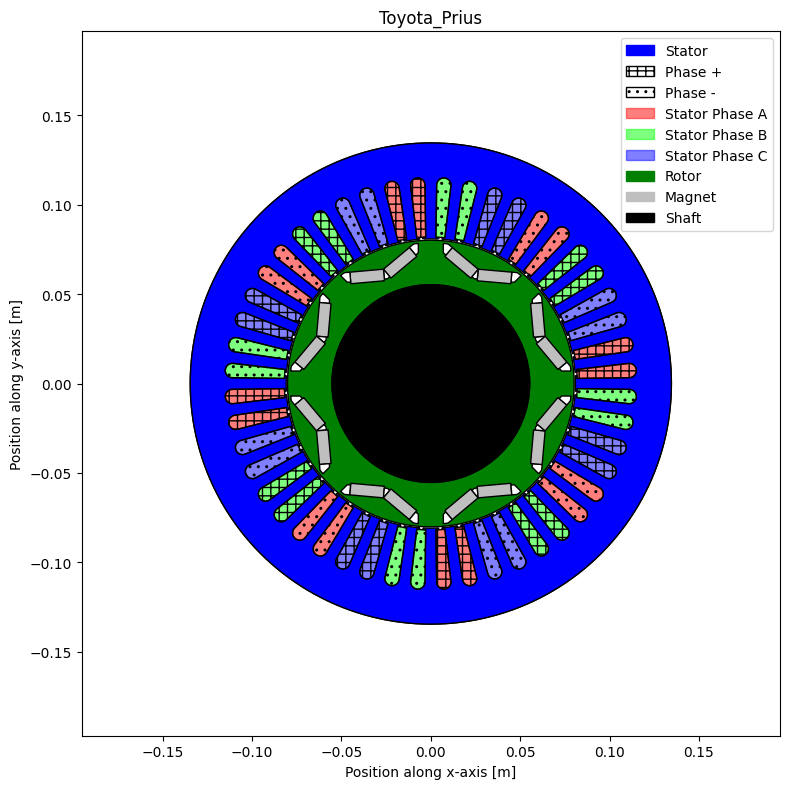
Every electrical machine defined in Pyleecan can be automatically drawn in FEMM to compute torque, airgap flux and electromotive force.

Defining or loading the machine

The first step is to define the machine to simulate. For this tutorial we use the Toyota Prius 2004 machine defined in this tutorial.

%matplotlib inline

# Load the machine
from os.path import join
from pyleecan.Functions.load import load
from pyleecan.definitions import DATA_DIR

IPMSM_A = load(join(DATA_DIR, "Machine", "Toyota_Prius.json"))
# In Jupyter notebook, we set is_show_fig=False to skip call to fig.show() to avoid a warning message
# All plot methods return the corresponding matplotlib figure and axis to further edit the resulting plot
fig, ax = IPMSM_A.plot(is_show_fig=False)

Simulation definition

Inputs

The simulation is defined with a Simu1 object. This object corresponds to a simulation with 5 sequential physics (or modules): - electrical

- magnetic

- force

- structural

- losses

Each physics/modules can have several models to solve them. For now pyleecan includes: - an Electrical model with one Equivalent circuit for PMSM machines and one for SCIM. - a Magnetic model with FEMM for all machines - a Force model (Maxwell Tensor) - Magnetic and Structural models with GMSH/Elmer - Losses models (FEMM, Bertotti, Steinmetz)

Simu1 object enforces a weak coupling between each physics: the input of each physic is the output of the previous one.

The Magnetic physics is defined with the object MagFEMM and the other physics are deactivated (set to None).

We define the starting point of the simulation with an InputCurrent object to enforce the electrical module output with: - angular and the time discretization

- rotor speed

- stator currents

from os.path import join

from numpy import ones, pi, array, linspace, cos, sqrt

from pyleecan.Classes.Simu1 import Simu1
from pyleecan.Classes.InputCurrent import InputCurrent
from pyleecan.Classes.OPdq import OPdq
from pyleecan.Classes.MagFEMM import MagFEMM

# Create the Simulation
simu_femm = Simu1(name="FEMM_simulation", machine=IPMSM_A)
# simu_femm.path_result = "path/to/folder" Path to the Result folder to use (will contain FEMM files)
p = simu_femm.machine.stator.winding.p
qs = simu_femm.machine.stator.winding.qs

# Defining Simulation Input
simu_femm.input = InputCurrent()

# Rotor speed [rpm]
N0 = 3000
simu_femm.input.OP = OPdq(N0=N0)

# time discretization [s]
time = linspace(start=0, stop=60/N0, num=32*p, endpoint=False) # 32*p timesteps
simu_femm.input.time = time

# Angular discretization along the airgap circonference for flux density calculation
simu_femm.input.angle = linspace(start = 0, stop = 2*pi, num=2048, endpoint=False) # 2048 steps

# Stator currents as a function of time, each column correspond to one phase [A]
I0_rms = 250/sqrt(2)
felec = p * N0 /60 # [Hz]
rot_dir = simu_femm.machine.stator.comp_mmf_dir()
Phi0 = 140*pi/180  # Maximum Torque Per Amp

Ia = (
    I0_rms
    * sqrt(2)
    * cos(2 * pi * felec * time + 0 * rot_dir * 2 * pi / qs + Phi0)
)
Ib = (
    I0_rms
    * sqrt(2)
    * cos(2 * pi * felec * time + 1 * rot_dir * 2 * pi / qs + Phi0)
)
Ic = (
    I0_rms
    * sqrt(2)
    * cos(2 * pi * felec * time + 2 * rot_dir * 2 * pi / qs + Phi0)
)
simu_femm.input.Is = array([Ia, Ib, Ic]).transpose()

In this example stator currents are enforced as a function of time for each phase. Sinusoidal current can also be defined with Id/Iq as explained in this tutorial.

MagFEMM configuration

For the configuration of the Magnetic module, we use the object MagFEMM that computes the airgap flux density by calling FEMM. The model parameters are set though the properties of the MagFEMM object. In this tutorial we will present the main ones, the complete list is available by looking at Magnetics and MagFEMM classes documentation.

type_BH_stator and type_BH_rotor enable to select how to model the B(H) curve of the laminations in FEMM. The material parameters and in particular the B(H) curve are setup directly in the machine lamination material.

from pyleecan.Classes.MagFEMM import MagFEMM

simu_femm.mag = MagFEMM(
    type_BH_stator=0, # 0 to use the material B(H) curve,
                      # 1 to use linear B(H) curve according to mur_lin,
                      # 2 to enforce infinite permeability (mur_lin =100000)
    type_BH_rotor=0,  # 0 to use the material B(H) curve,
                      # 1 to use linear B(H) curve according to mur_lin,
                      # 2 to enforce infinite permeability (mur_lin =100000)
    file_name = "", # Name of the file to save the FEMM model
    is_fast_draw=True,  # Speed-up drawing of the machine by using lamination periodicity
    is_sliding_band=True,  # True to use the symetry of the lamination to draw the machine faster
    is_calc_torque_energy=True, # True to calculate torque from integration of energy derivate over rotor elements
    T_mag=60,  # Permanent magnet temperature to adapt magnet remanent flux density [°C]
    is_remove_ventS=False,  # True to remove stator ventilation duct
    is_remove_ventR=False,  # True to remove rotor ventilation duct
)

# Only the magnetic module is defined
simu_femm.elec = None
simu_femm.force = None
simu_femm.struct = None

Pyleecan coupling with FEMM enables to define the machine with symmetry and with sliding band to optimize the computation time. The angular periodicity of the machine will be computed and (in the particular case) only 1/8 of the machine will be drawn (4 symmetries + antiperiodicity):

simu_femm.mag.is_periodicity_a=True

The same is done for time periodicity only half of one electrical period is calculated (i.e: 1/8 of mechanical period):

simu_femm.mag.is_periodicity_t=True

Pyleecan enable to parallelize the call to FEMM by simply setting:

simu_femm.mag.nb_worker = 4  # Number of FEMM instances to run at the same time (1 by default)

At the end of the simulation, the mesh and the solution can be saved in the Output object with:

simu_femm.mag.is_get_meshsolution = True # To get FEA mesh for latter post-procesing
simu_femm.mag.is_save_meshsolution_as_file = False # To save FEA results in a dat file

Run simulation

out_femm = simu_femm.run()

[14:07:00] Starting running simulation FEMM_simulation (machine=Toyota_Prius)
[14:07:00] Starting Magnetic module
[14:07:01] Computing Airgap Flux in FEMM
[14:07:05] End of simulation FEMM_simulation

When running the simulation, an FEMM window runs in background. You can open it to see pyleecan drawing the machine and defining the surfaces. The simulation will compute 32*p/8 different timesteps by updating the current and the sliding band boundary condition. If the parallelization is activated (simu_femm.mag.nb_worker >1) then the time steps are computed out of order.

Once the simulation is finished, an Output object is return. The results are stored in the magnetic part of the output (i.e. out_femm.mag ) and different plots can be called. This out_femm.mag contains:

- Time: magnetic time axis

- Angle: magnetic position

- B: airgap flux density (contains radial and tangential components)

- Tem: electromagnetic torque

- Tem_av: average electromagnetic torque - Tem_rip_pp : Peak to Peak Torque ripple - Tem_rip_norm: Peak to Peak Torque ripple normalized according to average torque

- Phi_wind_stator: stator winding flux

- emf: electromotive force

Some of these properties are “Data objects” from the SciDataTool project. These object enables to handle unit conversion, interpolation, fft, periodicity…

Plot results

Output object embbed different plots to visualize results easily. A dedicated tutorial is available here.

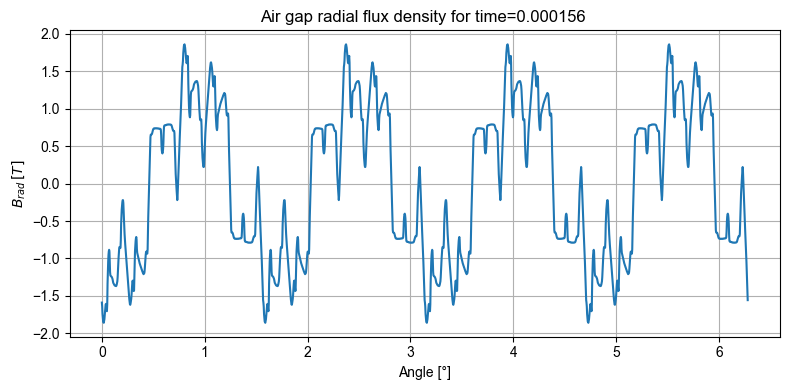
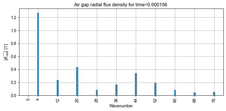
For instance, the radial and tangential magnetic flux in the airgap at a specific timestep can be plotted with:

# Radial magnetic flux
out_femm.mag.B.plot_2D_Data("angle","time[1]",component_list=["radial"], is_show_fig=False)
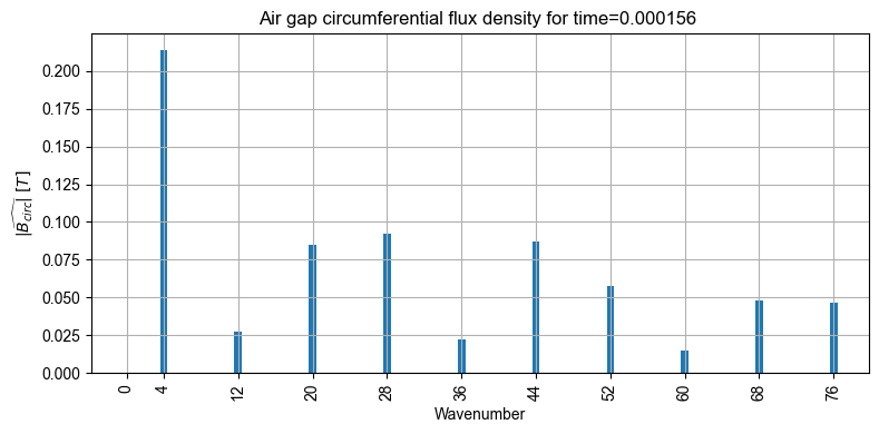
out_femm.mag.B.plot_2D_Data("wavenumber=[0,76]","time[1]",component_list=["radial"], is_show_fig=False)

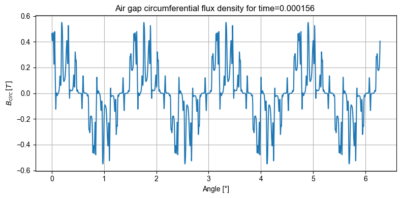
# Tangential magnetic flux
out_femm.mag.B.plot_2D_Data("angle","time[1]",component_list=["tangential"], is_show_fig=False)
out_femm.mag.B.plot_2D_Data("wavenumber=[0,76]","time[1]",component_list=["tangential"], is_show_fig=False)

The torque can be plotted with:

out_femm.mag.Tem.plot_2D_Data("time", is_show_fig=False)

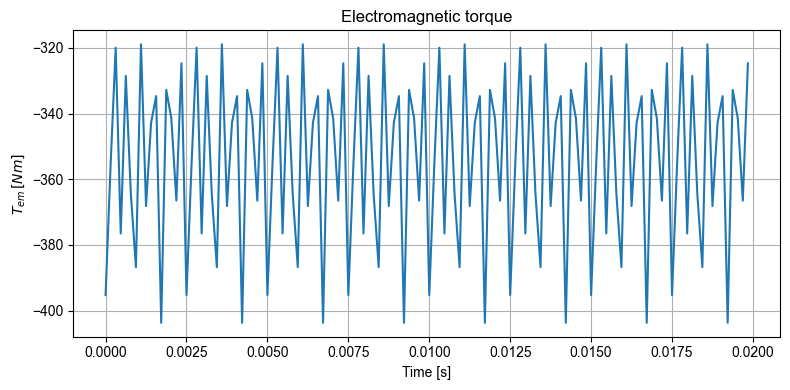
One can notice that the torque matrix includes the periodicity (only the meaningful part is stored)

print(out_femm.mag.Tem.values.shape)
print(simu_femm.input.Nt_tot)

(16,)
128

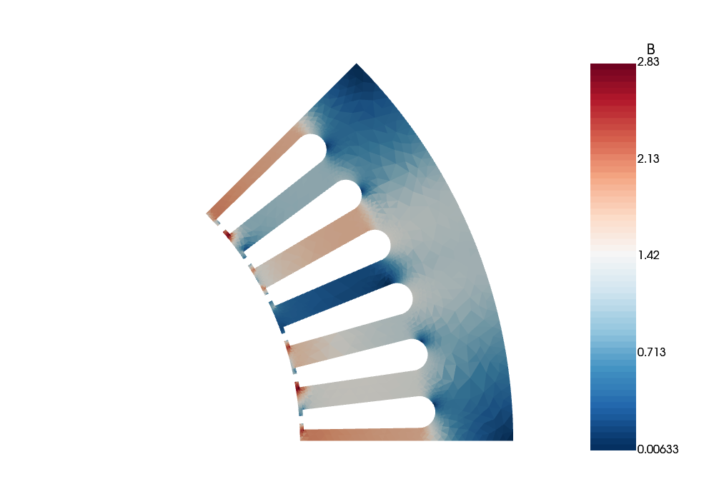
If the mesh was saved in the output object (mySimu.mag.is_get_meshsolution = True), it can be plotted with:

out_femm.mag.meshsolution.plot_contour(label="B", group_names="stator core", clim=[0,3])

WARNING:root:VTK requires 3D points, but 2D points given. Appending 0 third component.

Finally, it is possible to extend pyleecan by implementing new plot by using the results from output. For instance, the following plot requires plotly to display the radial flux density in the airgap over time and angle.

#%run -m pip install plotly # Uncomment this line to install plotly
import plotly.graph_objects as go
from plotly.offline import init_notebook_mode
init_notebook_mode()

result = out_femm.mag.B.components["radial"].get_along("angle{°}", "time")
x = result["angle"]
y = result["time"]
z = result["B_{rad}"]
fig = go.Figure(data=[go.Surface(z=z, x=x, y=y)])
fig.update_layout( )
fig.update_layout(title='Radial flux density in the airgap over time and angle',
                  autosize=True,
                  scene = dict(
                      xaxis_title='Angle [°]',
                      yaxis_title='Time [s]',
                      zaxis_title='Flux [T]'
                  ),
                  width=700,
                  margin=dict(r=20, b=100, l=10, t=100),
                 )

fig.show(config = {"displaylogo":False})